If your business ( or even your personal life ) requires you to do anything hearty with number , chances are you habituate a spreadsheet app to do it . As a Mac user , you ’ve drive plenty of choices among spreadsheet apps , but for most of us the choice come in down to three : Microsoft ’s Excel 2011;Apple ’s Numbers ( reading 3.2 ) ; and the web browser app - found Sheets section of Google Docs .
The one to use is really a personal selection , and that decision is not the focusing of this article . ( I personally favor Excel , mayhap becauseI’ve been using it for nearly 30 years ) . But no matter of the app you use , the interrogative sentence here is : How well do you know how to use it , really ?
As a spreadsheet vet , I devote that motion some thought and came up with the follow listing of thing that I think every savvy spreadsheet jockey — not novice , but people who ’ve been using one of these apps for a while — should bang . I ’m not verbalize about any specific undertaking . Rather , these are the proficiency and concept that I think you should love for calibrate from cursory to serious user .
1. Format Numbers
Because numbers can take many forms ( decimals , integers , portion ) , you need to apply format to make it clear what they imply . For example , most people would find it well-heeled to understand 25 % as opposed to 0.25 . So , after you insert the number in a cell and select that cellular telephone :
surpass : Many often - used number arrange options are visible in the Home ribbon . you may also expend the Format > Cells menu , then click Number in the dialogue box that appears . All turn data format are listed down the remaining edge of the duologue box ; prize one , and its choice appear on the right hand .
The Custom option ( recently total to Numbers as well ) is especially useful , as you may unite text with your formatted number . For representative , a formatting of#,##0.00 " widgets"would format your act with a Polygonia comma if call for , two decimal places , and the wordwidgetsafter the number . Your cells will still be treated as numbers for use in deliberation , but they will display with the defined textual matter .
Numbers : Click the Format icon ( the paintbrush ) in the toolbar , then take the Cell entry in the resulting sidebar . Select the option ( reflexive , Number , and so on ) you want to utilise from the pop - up carte du jour . You may take to set other value : For exemplar , if you prefer Numeral System , you ’ll demand to adjust value for Base , Places , and how to represent negative identification number . ( Numbers also include limited number formats such as Slider , Stepper , pa - up Menu , and more ; these can be used to make intuitive data introduction forms . )
Numbers put up a clustering of specialized numeral data formatting , include Slider .
Sheets : All number formats can be feel in the Format > Number fare ; each formatting option appears in its own hierarchical menu . As in Excel , you could make custom number formats that immix schoolbook and numbers — but you have to chance the option first , as it ’s bury in the Format > turn > More Formats submenu .
2. Merge Cells
Another useful formatting trick is to merge cells . integrated cell are what they sound like : two or more cells unite into one . This is a bang-up direction to revolve about a header above a routine of editorial , for exemplar . incorporate cells are a knock-down way to get away from the strict column - and - row layout of a typical spreadsheet .
To merge cells , you require to have a value only in the first cell you intend to merge , as values in any other cubicle will be wiped out by the merge . Select the reach of cells to merge , by clicking on the first cell ( the one take the data ) and dragging through the range you wish to merge .
stand out : snap the Merge entry in the Home ribbon , and then select one of the Merge options that appear in the pour down - up menu — Merge and Center is what I employ most often .
Numbers : Select tabular array > Merge Cells .
unite two cells into one is handy for creating chromatography column header .
Sheets : Select Format > Merge Cells , then prefer one of the Merge options , such as Merge Horizontally .
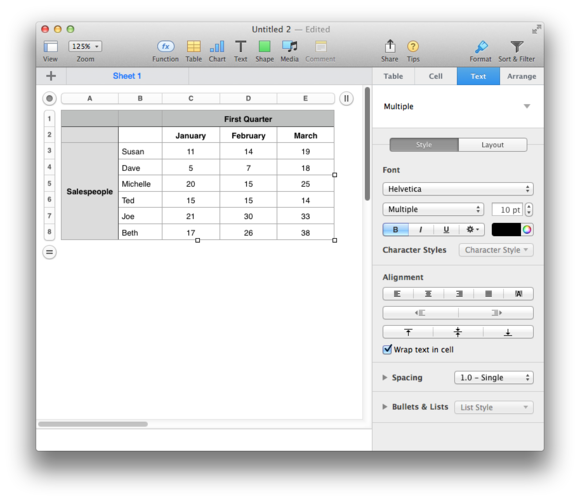
you’re able to also unite cell vertically , which can be utile in table where you have a parent cell ( Salesperson , for instance ) that contains multiple course of data point ( for exercise , merchandise sell and Units Sold ) .
3. Use Functions
You believably already know how to use basic formula to do basic arithmetic on cellular telephone content . Butfunctions , which get you manipulate text and numbers in many other way , are how you really unlock the potential of spreadsheets .
If quantity count most , then Excel would acquire , with ( if I counted correctly ) 398 unique functions . Google Sheets comes in a close second with 343 , and number has 282 . But the total count is irrelevant , as long as the app has the functions you need .
All three apps deal a large set of commonly used functions . For example , to add up numbers across a range of cells , they all put up = SUM(RANGE)(whereRANGEis a reference book to the range of cells to be summed in the parentheses ) . To feel the norm of a range of number , they have = AVERAGE(RANGE ) . To round off a number to two denary places , you may practice = ROUND(CELL,2 ) .
With 250 - plus functions in each app , there ’s no fashion I can depict even a reasonable portion of them . But here are some of the less - obvious single that I apply all the time ; they also happen to be in the same soma in all three apps :
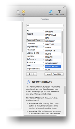
Numbers ’ ready to hand function web browser .
= COUNT ( ): count all numeric incoming in a range . Nonnumeric values will be skip over . To let in nonnumeric values , apply = COUNTA(RANGE)instead .
= MAX(RANGE)and = MIN(RANGE ): Return the largest and modest value in a range . interrelate to these two , I also often apply = RANK(CELL , RANGE ) , which return the rank and file of a given cell within the specified cooking stove .
= NOW : Inserts the current escort and time , which is then update each metre the spreadsheet recalculates . ( In both Excel and Sheets , you require to add together a set of parentheses:=NOW ( ) . )
= TRIM(CELL ): If you play with text that you copy and paste from other generator , there ’s a good chance you ’ll find extra spaces at the commencement or end of some pedigree of text . The TRIM function transfer all those lead and go after spaces but leaves the blank space between words .
Beyond these examples , the well way to get to know the functions in each app is to dally around with its mathematical function web browser app . In Numbers , you ’ll see the internet browser as soon as you type an equal foretoken ( =) ; it appears in the right sidebar and provides a nice verbal description and instance of each function . In Excel , select View > Formula Builder ( in the Toolbox ) . In plane , quality Help > Function List , which merely get to the Sheets web page showing the tilt of functions .
4. Distinguish Between Relative and Absolute References
In the functions listed above , CELLandRANGEare references to either an individual cellphone or a mountain range of cell . So = ROUND(C14,2)will take the note value in cubicle C14 and flesh out it off to two digits;=SUM(A10 : A20)will add up all the number in cells A10 through A20 .
you’re able to embark these electric cell locations either by typing them or by dawn ( or , for ranges , sink in and dragging ) the mouse .
Spreadsheet apps are also quite smart ; if you replicate = SUM(A10 : A20)and paste it into the column to the right , it will mechanically shift to = SUM(B10 : B20 ) . This is calledrelative addressing , as the functions ’ table of contents are relative to where they ’re range ; it ’s the nonremittal for formulas in all three apps .
If you do n’t want the cell references to change when you simulate or move a formula , all three apps offer a mode calledabsolute addressing . An downright address does n’t change when copy to a new location . All three apps utilize the same symbol for creating one : a dollar signaling before the quarrel and/or column symbol in a formula . So instead of typingA10 : A20 , for model , you type$A$10:$A$20to make a fixed rule that always refers to those cells , regardless of where you put it .
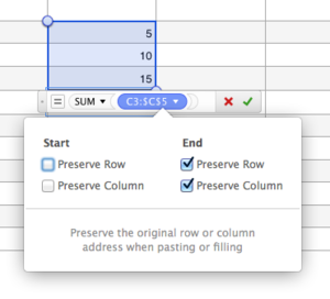
number ’ out-and-out / relative cellphone - addressing windowpane .
you could also lock only one direction : $ A10:$A20 will always refer to column A , but if you copy the convention over one column and down 50 rows , it would change to $ A60:$A70 . Similarly , A$ 10 : A$20 would lock the rows ; re-create this expression over one and down 50 , and it would change to B$10 : B$20 .
If you ’re typewrite cell addresses directly , all three apps get you simply type the dollar sign manually . But if you ’re pick out cells with chink and drags , Numbers has another path of switching between relative and absolute addressing .
electric cell reference work tot via click and drag seem in small colored bubbles , with a triangle to the right ; you sink in the triangle to pop up Numbers ’ inviolable / relative cubicle - speak window . But while this method acting works , I notice it more time - consume than merely typing the dollar house where I want them to be .
5. Name Cell References
Referring to cell by emplacement may be convenient , but it can also make it voiceless to figure out precisely what a given formula is doing . It also signify you call for to remember the positioning of often - used cells , which can be tricky in a large spreadsheet . If you name cell ( and range ) , however , you’re able to make the formula easy to read , as well as make recycle those cells in other rule easier .
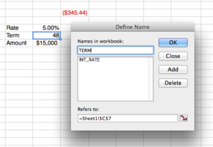
Consider this pattern as an example:=PMT(C5/12,C6,C7 ) . Just by reading it , you’re able to probably guess that it return a payment of some sort , and peradventure you’re able to tell that cell C5 contain an annual pastime pace . But really , it ’s not gentle to discern what this convention is doing . Here ’s the same formula using named cells:=PMT(INT_RATE/12,TERM , LOAN_AMT ) . Now it ’s a lot exonerated what ’s going on , and you no longer need to remember that cell C5 is the annual involvement pace .
Naming stove in Excel .
Excel : take the cellular telephone or straddle you ’d like to name , then select Insert > Name > Define , which will come out up a young window . Type the name you ’d wish to create in the first loge , then click Add . Repeat for as many names as you ’d like to define . Once you ’ve defined all your names , Excel even provides a way to utilize them to exist functions . Select Insert > Name > enforce , and you ’ll get a small window showing all your name cells and ranges . Hold down the < displacement > headstone , select the first name in the leaning , then click the last name in the lean to select them all . Click OK , and Excel will insert the epithet into any function that references a discover cellphone or chain .
Once you ’ve bring up a cellular phone or range , the spreadsheet always uses it in formulas — even if you select a cell , Excel will tuck its name in the formula .
Numbers : Sadly , it does n’t support named ranges .
sheet : choose the cell or range you ’d like to name , then select Data > make Range . This will display a sidebar where you may typewrite the name of the chain and ( if necessary ) change the prison cell reference . Click Done , and you ’ve make a named range ( even if it ’s just one cell ) . I ’m not mindful of any path to apply freshly create name calling to be formulas . Unlike Excel , flat solid wo n’t use a name unless you specifically typewrite it in .
6. Extract Data From Ranges
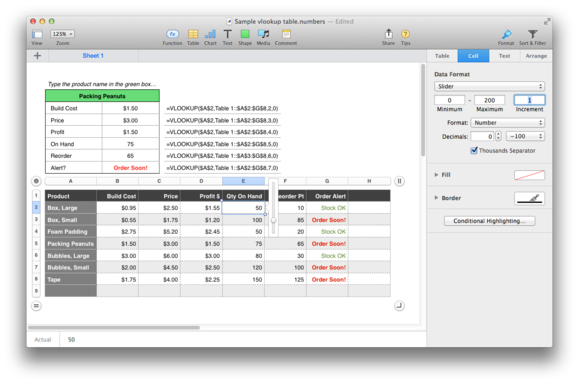
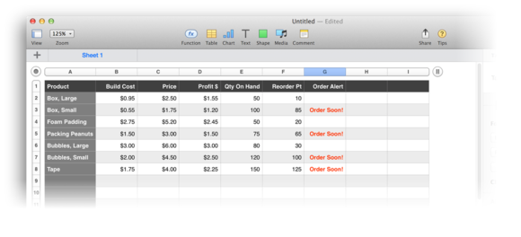
One of the most - common uses of a spreadsheet is to create tabular data and then distill value from that datum . weigh the play along worksheet for a company that sell shipping supply :
Your occupation is to answer coworkers ’ queries , such as “ What ’s our cost on the packing peanuts ? ” and “ How many roll of taping do we have on deal ? ” You could , of trend , just look at the mesa every time someone asked a question , but take that the real - universe variation of the table may have hundreds or one thousand of rows . There has to be a near way .
And there is : TheVLOOKUPandHLOOKUPfunctions pull data out of tables , by cope with a lookup time value to a economic value in the mesa . ( These part are monovular in all three apps , so I ’ll explain how they knead in Numbers . )
VLOOKUPis used when your data point is as shown in the table above : each point is on its own row , with multiple column of associated data . HLOOKUPis used when each item is in its own newspaper column , with multiple row of associated data point .
The layout of the pattern is the same in each app :
VLOOKUP(LOOKUP_VALUE , COLUMN_NUMBER ( ROW_NUMBER for HLOOKUP ) TO RETURN , REQUIRE EXACT MATCH )
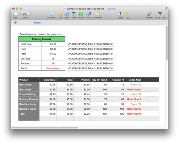
Using a fewVLOOKUPformulas , you may produce a lookup instrument to quickly come back all the data point about a given product . Here ’s the same worksheet as above , but with a product - search board added to the top . I ’ve also include the actual formulas that are generating the termination , so you’re able to see howVLOOKUPworks .
As one example , here ’s the formula in the On Hand wrangle : VLOOKUP($A$2,Table 1::$A$2:$G$8,5,0 )
$ A$ 2is an out-and-out reference to the time value to match in the table — the subject of the green box , in other words . tabular array 1::$A$2:$G$8is the range of cells in which number will search for a match for whatever ’s in$A$2 . ( This is a great model of why naming ranges would be handy in Numbers . ) The5tells Numbers to take back the time value in the fifth pillar ( the first column is pillar one ) ; this is the tower that deem the quantity on bridge player .
Finally , that dog zero is very of import : It distinguish the spreadsheet to come back only exact match . If you pass on that off either lookup pattern , figure will returnfuzzy match — catch that number close to matching the search value . In this suit , that would be speculative — if you make a erratum in your lookup cell , you do n’t want to see a nearly fit production , you want to see error messages , lease you know there was something wrong with the lookup .
The other formulas are fundamentally monovular , differ only in which column number ’s data is returned .
7. Perform Logical Tests
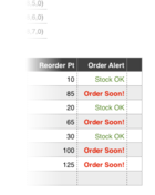
Many times , you take to define a cubicle ’s note value free-base on the results of one of more other cell values . For instance , in the worksheet for the merchant marine supplies company , the Order Alert column is either clean ( if there ’s mess of line of descent on hand ) or it contains theOrder Soon!warning ( when inventory is getting low ) .
How can one cellphone exhibit two possible values ? By using a legitimate function . Each of these spreadsheet apps includes a telephone number of logical functions ; the three peculiarly utilitarian 1 below appear in all three apps .
The first one lets you sum issue based on whether or not they satisfy a condition you define.=SUMIF(TEST_RANGE , CONDITION , OPTIONAL_SUM_RANGE)(If you leave outOPTIONAL_SUM_RANGE , thenTEST_RANGEis also used as the range of values to total . )
As an representative , using the worksheet for the shipping supplies ship’s company , this formula will total the Qty On Hand column , adding only those particular for which the Profit is more than $ 2.25:=SUMIF(D2 : D8,">2.25",E2 : E8 ) .
In this formula , the Profit column ( D2 : D8 ) is compared to the test ( is the value expectant than2.25 ? ) ; if it ’s greater , then the amount in column E ( E2 : E8 ) is added to the sum .
The 2d function , SUMIFS , is link up toSUMIF , but can take many optional pairs of trial range and conditions:=SUMIFS(SUM_RANGE , TEST_RANGE , CONDITION1,TEST_RANGE2,CONDITION2 , etc . ) .
For example , if you need the full quantity on deal for detail with profit over $ 2.25andbuild cost under $ 3.00 , it would look like this:=SUMIFS(E2 : E8,D2 : D8,">2.25",B2 : B8,"<3 " ) . The convention will sum the Qty On Hand column ( E2 : E8 ) , but only if both the profit ( D2 : D8 ) is over $ 2.25 ( " > 2.25"),andif the Build Cost ( B2 : B8 ) is under $ 3.00 ( " <3 " ) .
The third ( and , for me , most often - used ) logical function you should know how to use is the simpleIFfunction . UsingIFis a cracking way to vary cubicle results based on conditions being met or not being met . The sentence structure is pretty simple:=IF(CONDITION , RESULT_IF_TRUE , RESULT_IF_FALSE ) .
As one illustration , see the worksheet of the shipping supplying company ; the Order Alert column consist of nothing butIFstatements that all look like this one from cell G2:=IF(E2 / F2<1.25,“Order Soon ! " , " " ) .
The condition being tested is whether or not the proportion of the number of item on hired man to the reorder point is less than1.25(125 percent ) . If it is , it ’s time to order , and the"Order Soon!“warning appears . If it ’s not , then all is fine , and we leave alone the cellular phone empty by specifying an empty string as the False result .
IFstatements can get very complicated , as they can be nestle and can include not just inactive schoolbook , but also references to other cells , or even ranges of cells .
8. Mix Text and Formula Results
In the section on routine initialise , I explain how to add up text to a custom number format ( in Excel and Sheets ; not in Numbers ) . While this works , there are other ways of mixing textual matter and numeric results , thanks tostring - basedformulas .
deliberate our hypothetical shipping supplies company again . wear you want to prepare a write up for direction , showing the full investment ( Build Cost 10 Quantity On Hand ) for a given product . Of of course you could chop-chop do the math and then type out an email with the details .
Instead of doing that yourself , though , you could have your spreadsheet app build the sentence for you :
“ The full investment in Tape is $ 262.50 ( we have 150 in livestock at $ 1.75 each ) . ”
To do this , you need a special case : the ampersand ( & ) . The ampersand can be used to join one pattern note value , including text strings , to another .
So , for object lesson , to build the condemnation above ( in any of the three apps ) , the normal would look like this :
= " The total investment in " & A8 & " is " & DOLLAR(B8*E8 ) & " ( we have " & FIXED(E8,0 ) & " in stock at " & DOLLAR(B8,2 ) & " each).“The whoremaster here is to use theDOLLARandFIXEDfunctions ; these convince numbers to text that looks like numeral ; theDOLLARversion function automatically formats in currentness , complete with the dollar bill sign .
9. Use Conditional Formatting
As covered in the beginning , you could format numbers , school text , and jail cell in all three of these spreadsheet apps . But all three share a restriction when using traditional formatting : once something is format , it retains that formatting regardless of what might happen to the data in the cellular phone . If you ’re creating the blood dividers in your table of data , this is n’t much of a problem . But if you ’re endeavor to spotlight a specific type of number ( when you get hold of the inventory - purchase order point , say ) , then fixed formatting is n’t much help .
That ’s when conditional formatting is really handy . It ’s just what it sounds like : format that change based on conditions you narrow . Numbers refers to this feature film as Conditional Highlighting , and you ’ll find it in the Cell tab of the Format sidebar . Both Excel and Sheets come to to it as Conditional Formatting , and you ’ll find it with that name in the Format menu of both apps .
Conditional format is a complex topic ; to fully explore it requires many more words than we have here . But as one exercise of what it can do for you , view theIFfunction object lesson , used earlier to fulfill in the Order Alert pillar . Instead of having the formula plainly display an alert when supplies are low , we can change the formula to expose a message stating that there ’s mass of stocktaking . That modification is simple:=IF(E2 / F2<1.25,“Order Soon!”,“Stock OK " ) .
Ideally , theOrder Soon!alert should be bold and red . But that does n’t make sensory faculty forStock OK ; that might be better rendered as light immature and not boldface . By create a conditional highlighting / arrange principle , it ’s possible to change the cell ’s format based on the value .
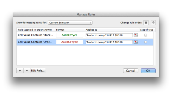
Excel : Select the cooking stove from G2 to G8 ( in this example ) , then take the Format > Conditional Formatting menu item . In the new window that appears , click the plus signaling ( to add a fresh normal ) . When the New Formatting Rule window appears , coif the Style pop music - up to Classic , which will open yet another windowpane ( that ’s three windows , and you have n’t even created a undivided dominion yet ) .
Conditional arrange in Excel .
In this newest window , leave the Style bulge - up set to Classic , then coiffure the second pop - up to Format Only Cells That Contain . Set the next two pop - ups to Specific Text and Containing , and then typeOrder Soon!in the text box . go under the Format With dada - up to Custom Format , which will open afourthwindow . select the Font tabloid , and set the Color pop - up to red , and clack the Bold entry in the Font Style boxful . check that nothing is filled in on the Border and Fill check , then click OK ( to shut the fourth window ) , and click OK again ( to shut the third ) .
Now do the same affair again , commence with the plus - sign click . But this metre , set the text edition box seat entry toStock OK , set the font color to green , and make trusted the font dash is normal , not bold . When you get back to the Manage Rules window , you should see both rules list ; click OK to ( finally ! ) give the rules .
The effect of conditional formatting in Numbers .
Numbers : take the range of cells ( G2 : G8 ) , then click the Conditional Highlighting button on the Cell tab key of the Format sidebar . This will vary the sidebar ; click the Add A Rule button to display a pop - up listing of rules , then click the Text tab . Click the Is entry , set the first pop - up to Text Is , and typeOrder Soon!in the loge . tick the Triangulum in the carte below the text entrance box , and select the final entry , Custom Style .
This will add yet another gore to the sidebar ; select a red tone in the color steering wheel , and select the B button for sheer text . ultimately , flick Done .
That formatting theOrder Soon!cells . But what about theStock OKmessages , which are soon just black text ? With the G2 : G8 range still choose , click Show Highlighting rule in the sidebar , then click Add a Rule again . Repeat the steps as above , except commute the school text corner to readStock OK , and set the custom expressive style to have nonbolded green text . Click Done , and you ’ll see both sheer red and normal immature text in the cell .
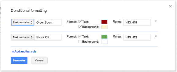
Sheets : choose the G2 : G8 range , then select the Format > Conditional Formatting menu item . In the dialog loge that seem , set the first papa - up to Text Contains , then typeOrder Soon!in the text box . Check the Text box to initialize the textual matter , then click the next on the face of it empty box to the right for display the vividness selector ; choose a nice shade of bolshy . You might also want to control the Background boxwood and lay out a desktop color ( bright jaundiced will get your attention ) , because sheet does n’t countenance you change the font ’s appearing with conditional data formatting .
Google Sheets ’ conditional formatting tool .
Click the Add Another Rule contact , and repeat the whole step , but typeStock OKin the text box , and use green for the text colour . After you ’ve set up the second normal , get through Save Rules to see the solution of your work .
